Bayesian networks for algorithmic thinking

Transforming data into information, knowledge, and wisdom - Part 1

This post was inspired by this presentation on data science.

During graduate school at UC Berkeley one of my favorite professors was Steve Selvin. I took most of his courses and bought most of his books. Steve introduced me to S-PLUS — the proprietary precursor of the open source R.¹ I came to love S-PLUS, and then R — a programming language and environment for statistical computing and graphics.² I used R for all my number-crunching — except for decision analysis! I was disappointed that R was not designed to construct decision trees like other software.³ I was determined to figure this out.

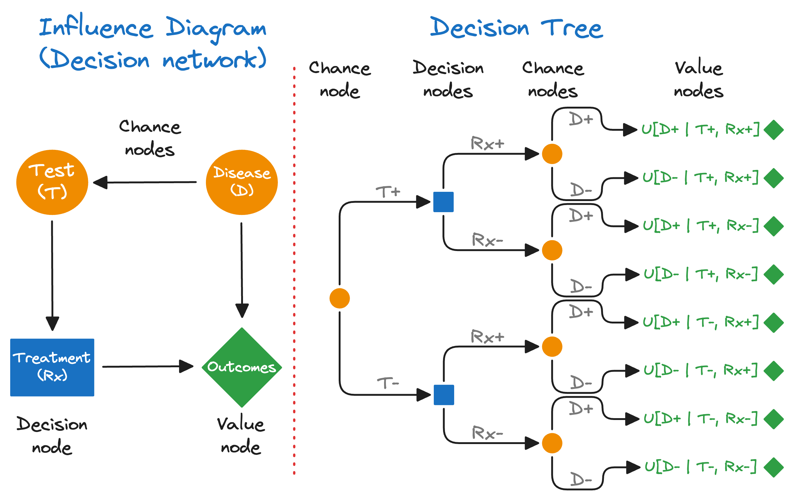
In 2015, I enrolled in Stanford’s certificate program in “Strategic Decision and Risk Management in Healthcare.” I learned a ton! I learned that decision trees (Figure 1, right) can be represented as influence diagrams (Figure 1, left).⁴ And that an influence diagram is also called a “decision network” — a type of “Bayesian network.” No, not “Bayesian statistics” but a Bayesian network! This really piqued my interest! It turns out that Bayesian networks — a type of probabilistic graphical model — could be implemented in R. I was thrilled!

Figure 1: Bayesian network equivalents: influence diagram (left), decision tree (left). Adapted from https://doi.org/10.1177/0272989X9701700301

Bayesian networks could be used not only for probabilistic reasoning, but also for causal inference and decision analysis! At the time, I was teaching R programming at UC Berkeley and I immediately integrated this into my course. A Bayesian network is the Swiss Army knife of population health thinking (which I now call Bayesian algorithmic thinking). Bayesian network concepts are easy to learn, promotes critical thinking, and are broadly applicable.

What is a Bayesian network?

A Bayesian network (BN) is a graphical model for representing probabilistic, but not necessarily causal, relationships between variables called nodes.⁵⁶ The nodes are connected by one-way arrows called edges. BNs have a superpower — they provide a unifying framework for understanding the following types of reasoning:

1. probabilistic reasoning (with Bayesian networks)

2. causal inference (with directed acyclic graphs)

3. decision analysis (with influence diagrams)

Nodes are just variables; eg, field names in a data table.

All public health professionals should understand basic Bayesian networks — starting with mastering two nodes (variables).

Consider this noncausal BN:

Smelling smoke indicates an increased probability of a fire burning nearby, but obviously smoke alone does not cause a fire. In other words, knowing X (smelling smoke) changes the credibility of Y (fire nearby). This can be formulated as a probability:

\(\Pr(\text{fire nearby} \mid \text{smell smoke})\)

In contrast, now consider this causal BN:

This causal BN depicts fire causing smoke. The causal arrow (edge) represents a unidirectional causal effect that can only point in direction. This specific causal network can also be expressed as a probability:

\(\Pr(\text{smoke} \mid \text{fire})\)

Notice that both noncausal and causal BNs have probabilistic dependencies, and that conditional probabilities arrows can always be formulated in both directions: eg, Pr(Y|X) or Pr(X|Y). In contrast, a causality arrow is always unidirectional.

To review: we have a Bayesian network with two variables (nodes) with a probabilistic relationship. And, we have a causal network (ie, a directed acyclic graph) which is a type of Bayesian network with a unidirectional, causal arrow.

Causal/predictive reasoning vs. evidential/diagnostic reasoning

Causal networks (DAGs) can be used for causal reasoning such as prediction:

Inferring causality comes natural to humans. In fact, we are quick to infer causality because we mistaken correlation for causation. For now, we will assume real causal effects. Causality enables prediction, but requires some effort. Fortunately, prediction can improve with practice, and in fact, is highly encourage.⁷ When a prediction disagrees with an outcome, we have prediction error. Closing the prediction error gap is called learning!

When a cause-effect relationship is not firmly established, the BN can represent the hypothesis-evidence concept:

We substituted “hypothesis” for “cause,” and “evidence” for “effect.” Notice that the probability of hypothesis given evidence, P(hypothesis|evidence), is the inverse probability of an effect given a cause: P(effect|cause).

In contrast to calculating P(effect|cause), that is used for causal/predictive reasoning, calculating P(hypothesis|evidence) requires Bayes’ theorem that is used for evidential/diagnostic reasoning. Whereas humans can become proficient at prediction calculations for causal/predictive reasoning, humans are terrible at calculating inverse probabilities using Bayes’ theorem for evidential/diagnostic reasoning.

Causal/predictive reasoning and evidential/diagnostic reasoning are used frequently in public health and medicine (Figure 2) — and sometimes not used!

Here are more public health examples:

Figure 2: Example of causal graphs in public health

DAGs can be used to estimate average causal effects which are not covered here. To learn about formal methods for causal influence, see Appendix for recommendations.

Bayes’ theorem for evidential/diagnostic reasoning

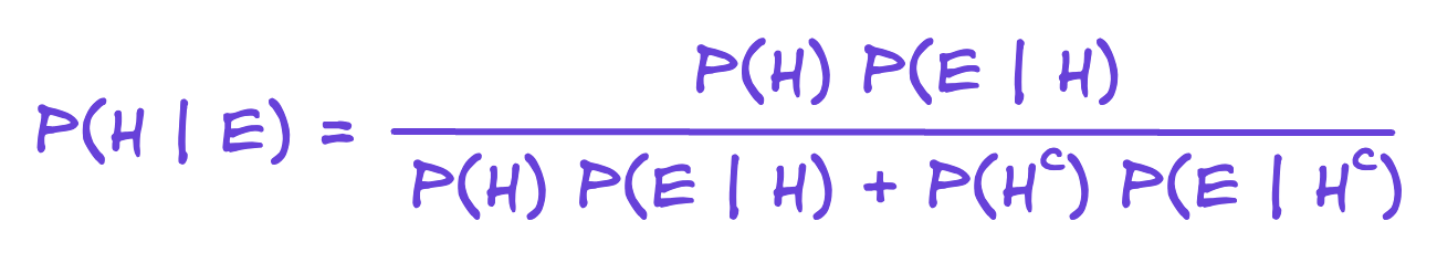
When we have a causal hypothesis (Does acetaminophen cause autism?) we use Bayes’ theorem to calculate the probability the hypothesis is credible given the evidence; ie, P(H | E), also called the posterior probability.

Figure 3: Bayes’ theorem

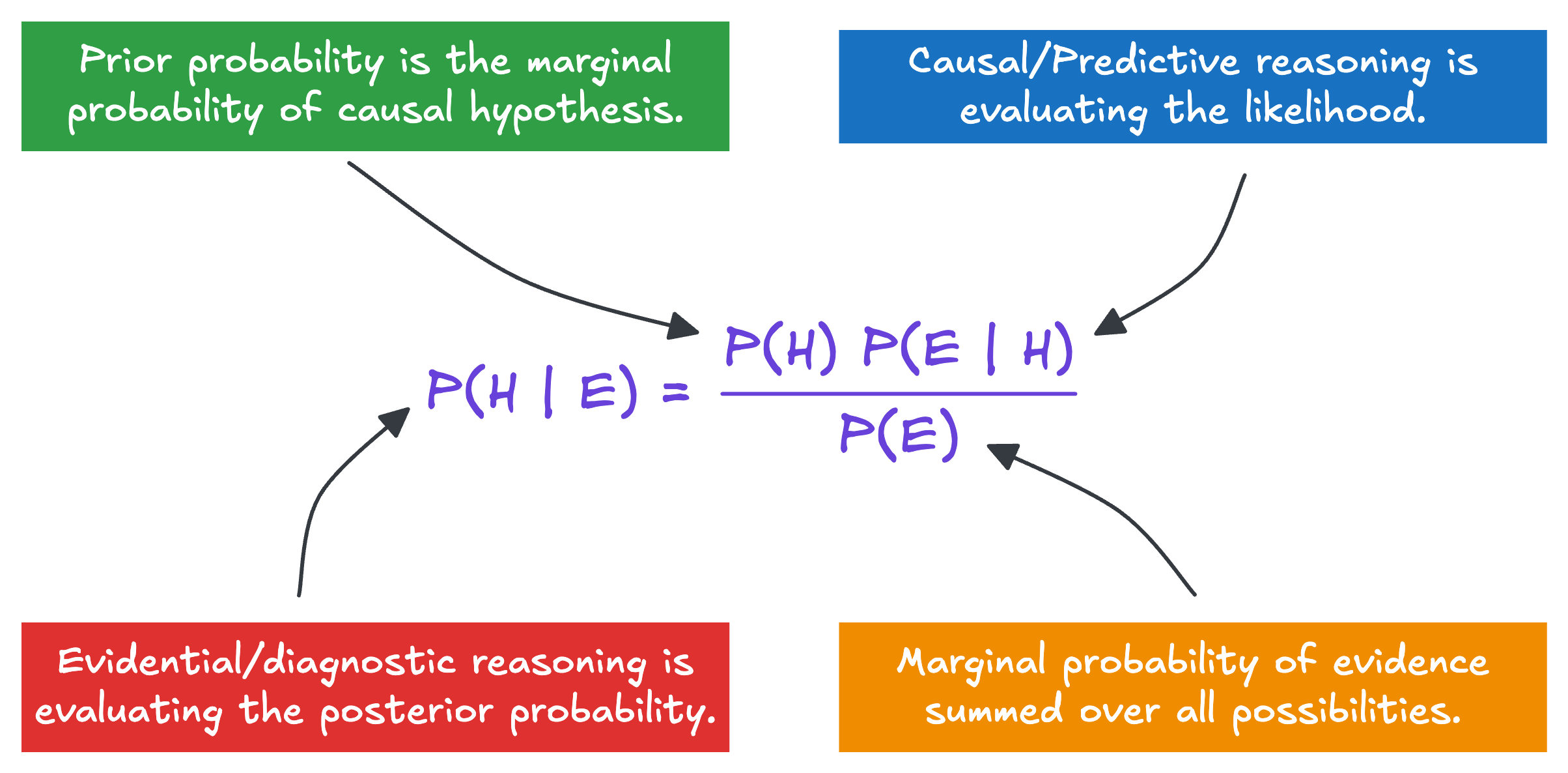
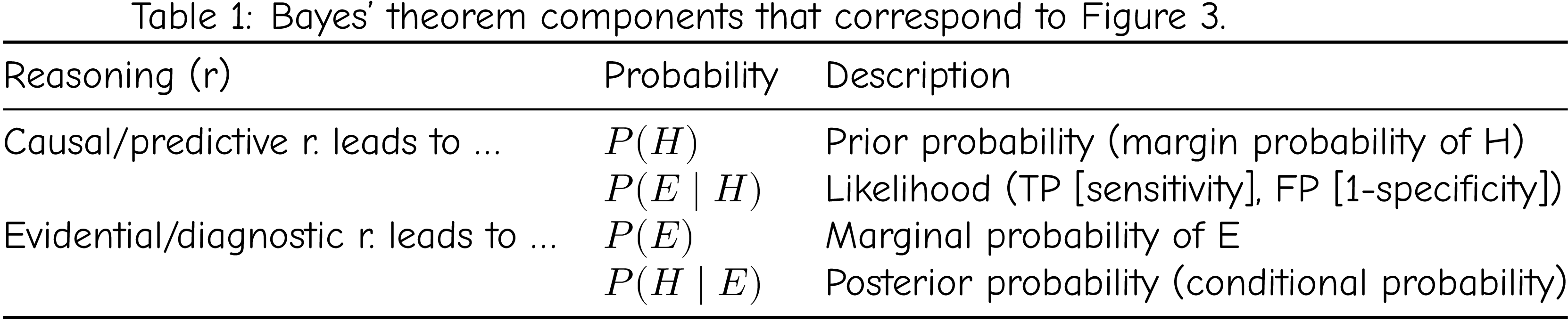
Bayes’ theorem is also used to quantify our subjective probabilities or beliefs. In Figure 3, P(H) is the prior (old) belief, P(H|E) is the posterior (new) belief, and P(E|H) is called the likelihood. The likelihood is critical because it is usually measurable, allowing us to update our belief. See Table 1.

The marginal probabilty P(E) can be “marginalized over H” which is a sum of conditional probabilities.

Bayes’ theorem is used to update

• probabilities (eg, risks of adverse events, diagnostic testing),

• credibility of a hypothesis (eg, evidence regarding causal claims), and

• beliefs (subjective beliefs).

Bayes’ theorem provides us with a systematic algorithm for processing evidence about a hypothesis.

• P(H|E) is the posterior probability: the probability the hypothesis is credible given the evidence.

• P(H) is the prior probability: the probability the hypothesis is credible before considering any evidence.

• P(E|H) is the likelihood: the accuracy of the evidence as a measure of the hypothesis (sensitivity, specificity, false positive, false negative, etc.)

  • sensitivity: the probability the evidence is present (eg, positive test) given the hypothesis is true (eg, disease present)

  • specificity: the probability the evidence is absent (eg, negative test) given the hypothesis is false (eg, disease absent)

A common application is using the results of a diagnostic test (evidence) to diagnose a disease state (hypothesis). For a worked out example see Richard Neapolitan, et al. “A Primer on Bayesian Decision Analysis With an Application to a Kidney Transplant Decision.” Transplantation 100, no. 3 (2016): 489–96. https://doi.org/10.1097/TP.0000000000001145. (also see⁸ )

Bayesian algorithmic thinking (BAT)

An alternative approach is to use Bayesian algorithmic thinking (BAT). From an individual agent’s perspective we have the following

• data (inputs: facts and signals from the internal and external environment)

• algorithms for processing data (cognitive, but can be computational)

  • causal reasoning (comes natural to humans)

  • evidential reasoning (requires Bayes’s theorem)

• inferences from algorithms

  • prediction (based on strength of causal reasoning)

  • diagnosis (based on strength of evidential reasoning)

Figure 4 is BAT for causal reasoning and prediction. An agent receives and processes data, applies an algorithm (causal reasoning), and generates an inference (prediction). This can happen automatically without our awareness. This is analogous to Daniel Kahneman’s System 1.⁹ Or, this can happen within our awareness with conscious intent, effort, and deliberation. This is analogous to Daniel Kahneman’s System 2. Causal reasoning and prediction comes natural to humans and improves with practice.

Figure 4: Bayesian algorithmic thinking — causal reasoning and prediction

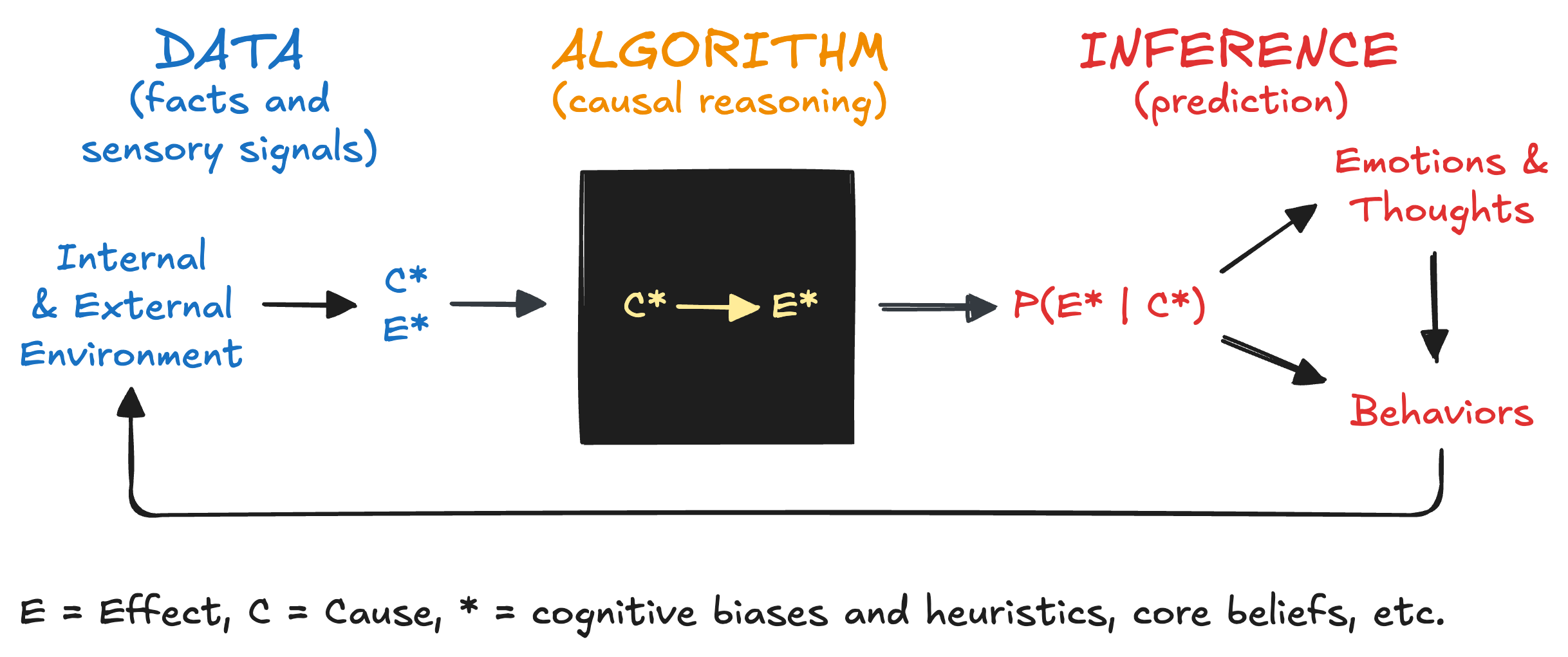
Figure 5 is BAT for evidential reasoning and diagnosis. An agent receives and processes data, applies an algorithm (evidential reasoning), and generates an inference (diagnosis). This can happen automatically without our awareness. This is analogous to Daniel Kahneman’s System 1. Or, this can happen with intent, effort, and deliberation within our awareness. This is analogous to Daniel Kahneman’s System 2. Evidential reasoning and diagnosis, done correctly, requires Bayes’s theorem. This process is much more challenging for humans.

Figure 5: Bayesian algorithmic thinking — Evidential reasoning and diagnosis

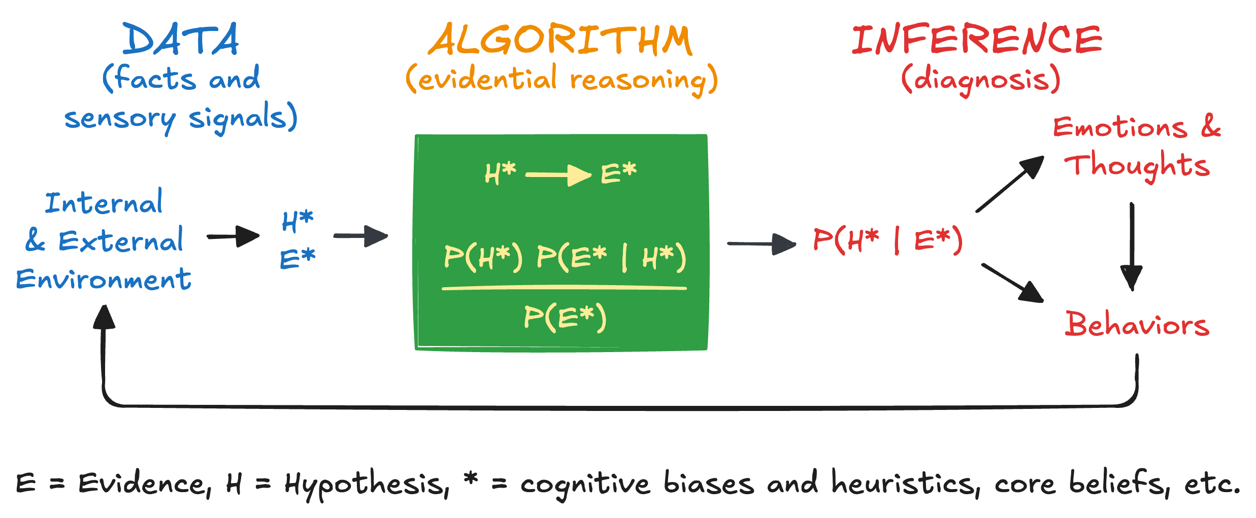
For BAT, we want to be aware of how our core beliefs, cognitive biases and heuristics, and psychological triggers impact

• posterior probabilities (think “hypothesis” and “evidence”),

• prior probabilities (baseline beliefs and credibilities), and

• likelihoods (ie, accuracy: true positives [sensitivity], false positives [1 - specificity]).

Be aware of the impacts on the thoughts, emotions, and behaviors of ourselves and others. We all learn as if we are applying Bayes’ theorem — but we are not. By embracing and deploying BAT, we will improve our reasoning skills.

CAUTION! Our System 1 brain actually predicts first using pre-existing causal models in our memory (ie, “priors”). If the prediction is not strongly refuted by the data; ie, the prediction error gap is small, the brain accepts the pre-existing causal model. This is energy efficient and preferred by our brains. If the prediction is strongly refuted by the data; ie, the prediction error gap is large, the brain has a “choice”: reject the pre-existing causal model, which is learning but requires energy, or stay with the pre-existing causal model, which is energy efficient but results in no learning. The brain learns by closing the prediction error gap.

Summary

In this blog we introduced Bayesian networks as a unifying framework for

• probabilistic reasoning,

• cause inference, and

• decision analysis.

We learned that with 2-variable causal graphs we can understand

• causal/predictive reasoning, and

• evidential/diagnostic reasoning.

Evidential/diagnostic reasoning requires Bayes’ theorem. As new data/evidence becomes available, Bayes’ theorem enables us to update

• probabilities (eg, risks of adverse events, diagnostic testing),

• credibility of a hypothesis (eg, new evidence regarding causal claims), and

• beliefs (subjective, personal beliefs).

Finally, Bayesian algorithmic thinking (BAT) allows us to generalize more broadly to the everyday processing of data (evidence), evaluating causality (hypothesis), and drawing conclusions (inference).

BAT will supercharge your critical thinking, keep you intellectually humble, and accelerate your learning and improvement.

In future posts, I will cover decision analysis, computation, and more than two nodes.

Thanks for supporting TEAM Public Health by reading this blog! Please share.

TEAM Public Health is a FREE — not-for-profit and reader-supported — blog. All content is freely available to all and is designed to be evergreen.

Serving with you,

Tomás

Appendix — Recommended

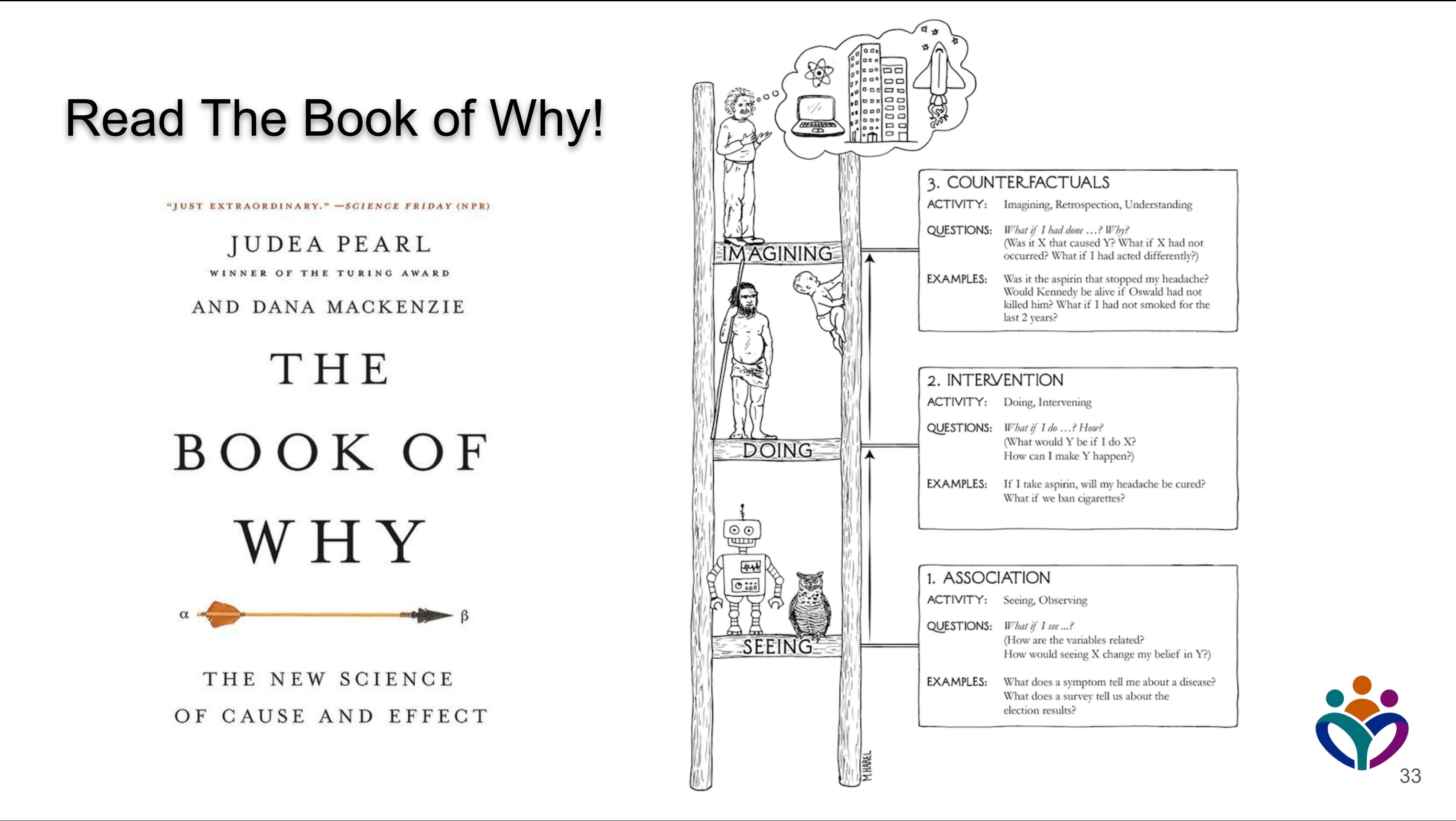
Read The Book of Why by Judea Pearl

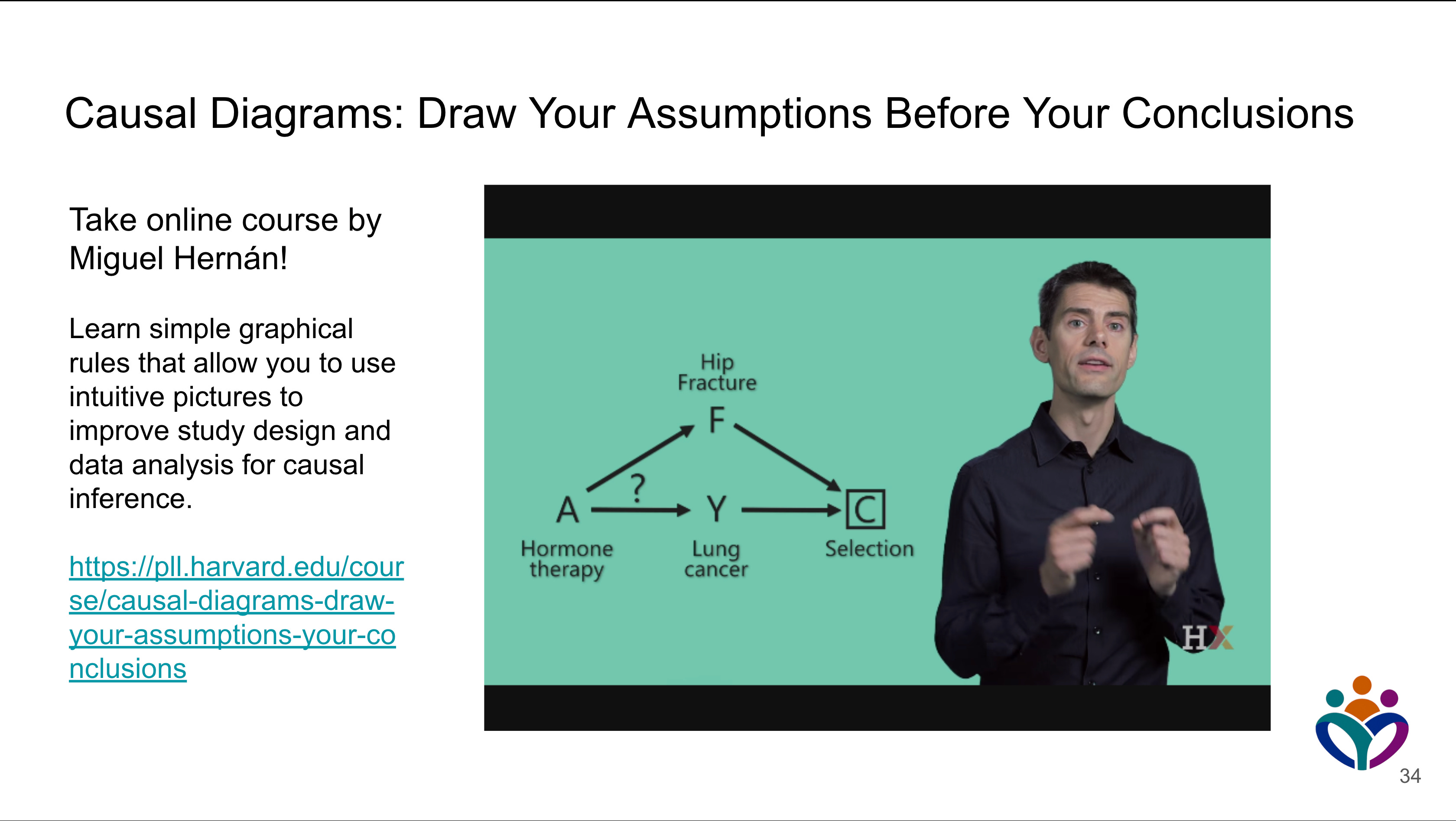
Take Professor Miguel Hernán’s course

https://pll.harvard.edu/course/causal-diagrams-draw-your-assumptions-your-conclusions

Read the causal roadmap article by LE Dang, et al.

Footnotes

1. https://www.r-project.org/

2. I started teaching R in 2004 before it was a popular programming language for data science.

3. See for example: https://www.treeage.com/, https://analytica.com/, https://www.syncopation.com/products/dpl-professional/, https://www.bayesia.com/

4. Owens, D. K., R. D. Shachter, and R. F. Nease. “Representation and Analysis of Medical Decision Problems with Influence Diagrams.” Medical Decision Making: An International Journal of the Society for Medical Decision Making 17, no. 3 (1997): 241–62. https://doi.org/10.1177/0272989X9701700301.

5. Scutari, Marco, and Jean-Baptiste Denis. Bayesian Networks: With Examples in R. Second edition. Texts in Statistical Science Series. CRC Press Taylor & Francis Group, 2022.

6. Fenton, Norman E., and Martin Neil. Risk Assessment and Decision Analysis with Bayesian Networks. Second edition. CRC Press, Taylor & Francis Group, 2019.

7. Moore, Don A. Perfectly Confident: How to Calibrate Your Decisions Wisely. 1st ed. HarperCollins Publishers, 2020.

8. Example calculation is also available here: Tomás J. Aragón. “Population Health Thinking with Bayesian Networks.” Preprint, eScholarship.org, December 8, 2019. https://escholarship.org/uc/item/8000r5m5.

9. Kahneman, Daniel. Thinking, Fast and Slow. 1st pbk. ed. Farrar, Straus and Giroux, 2013. https://us.macmillan.com/books/9780374533557/thinkingfastandslow.