Program theory is for the DAGs

Causality matters! Using causal graphs to explain your program interventions.

Every decision has causal and predictive assumptions. Based on these assumptions (often implicit), we make decisions and take actions towards our goals. Our public health programmatic activities are built upon these causal assumptions which collectively we call program theory. Every public health intervention has a program theory; however, many practitioners cannot describe the program theory supporting their primary programmatic activity or research. I too could not describe the program theories supporting my own work until I read Funnell Rogers’ book Purposeful Program Theory.¹

It turns out that program evaluators not only live and breathe program theory, but they call it by different names: logic model, program logic, theory of change, causal model, results chain, intervention logic, etc. Hence the confusion! From BetterEvaluation.org:

“A programme theory or theory of change (TOC) explains how an intervention (a project, a programme, a policy, a strategy) is understood to contribute to a chain of results that produce the intended or actual impacts.” 

In public health, the logic model is very popular. For me, a logic model is a good high-level summary for non-technical purposes (summary, communication, etc.); however, I do not like them (or variants) as a place to start. For me, program theory is for the DAGs — directed acyclic graphs² — and must include the theories of causation, change, and action.³

Program theory has three components and answers why? what? and how?:

1. theory of causation (Why? primary roots causes before an intervention),

2. theory of change (What? key strategies to affect the root causes), and

3. theory of action (How? key specific interventions to activate theory of change).

In public health we have two common DAG archetypes:⁴

1. a risk (adverse) event or condition and

2. a benefit (opportunity) event or condition (Figure 1).

For both, a trigger is an exposure, condition, activity, or incident that increases the probability of a risk or benefit event. A trigger can be a cumulative process. Before an intervention, these DAGs represent the theory of causation component of program theory.

Figure 1: Causal taxonomy for risk event (left) vs. benefit event (right)

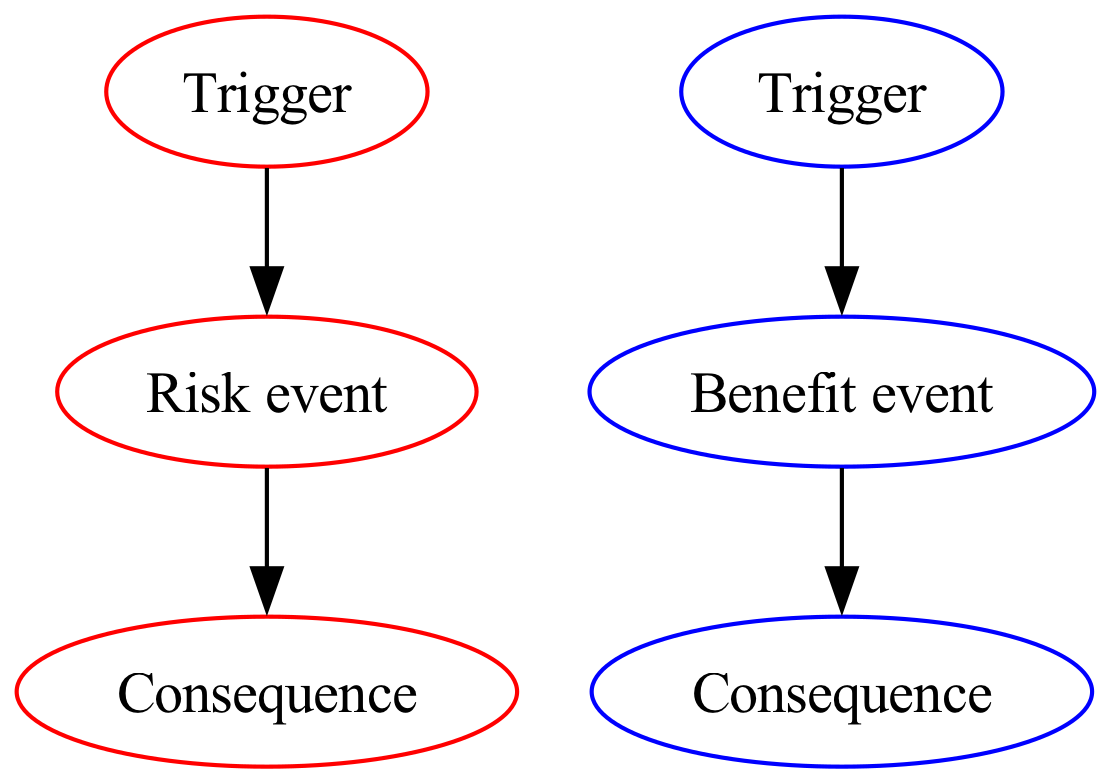
Figure 2 depicts the program theory for a public health intervention to reduce automobile crash injuries (a risk event). The theory of change has three strate- gies (prevention, control, and mitigation), and the theory of action has three interventions (speed bumps, automatic breaking, and seat belts).

Figure 2: Risk-reduction program theory: theory of causation, theory of change (strategy), and theory of action (intervention)

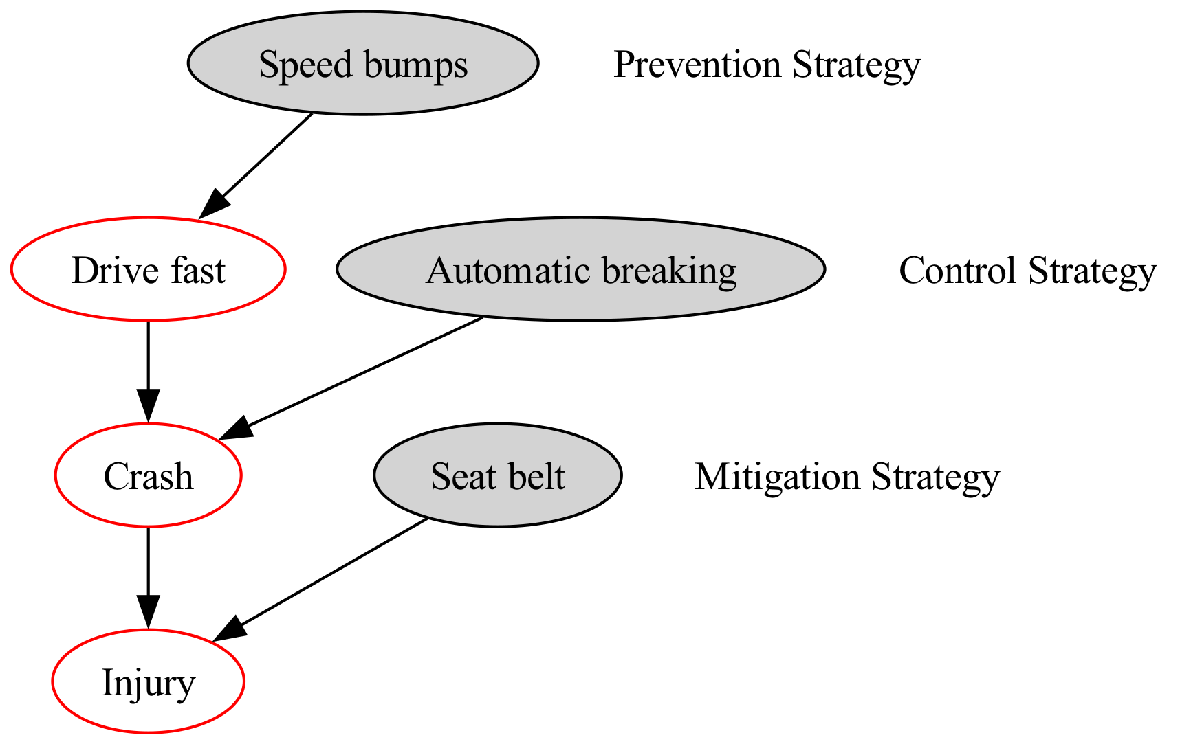
In a risk-event outcome (consequence), the 5 whys of root-cause analysis move backwards: Why was there an injury? Because of a crash. Why was there a crash? Because of fast driving? Why was there fast driving? We cannot answer this question (yet).

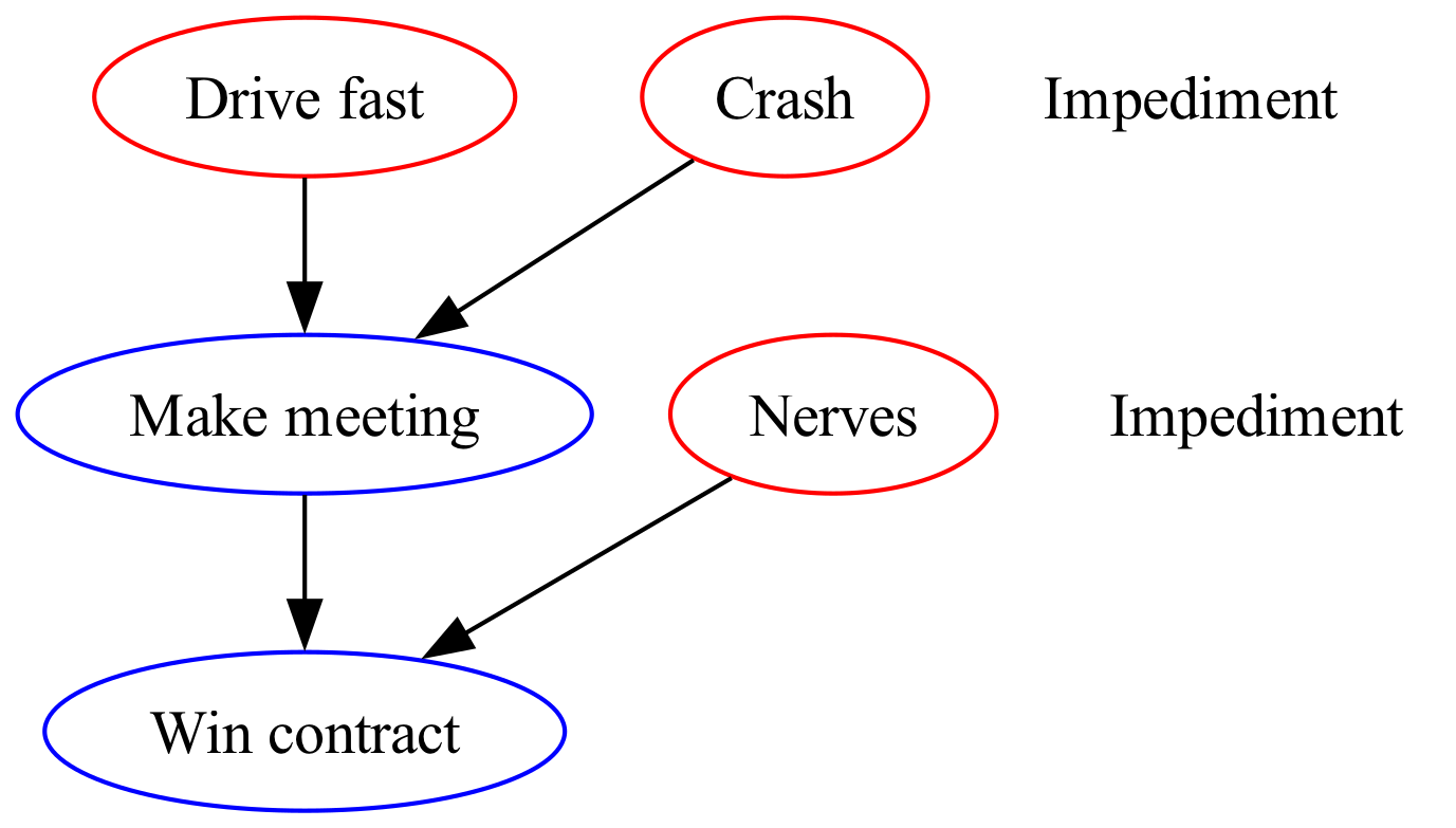
The program theory is not complete. We must also understand why people drive fast. We have not included the theory of causation from drivers’ perspective. Suppose, for instructional purposes, Figure 3 represents the most common DAG that explains why drivers speed. Therefore, why was he or she driving fast? To make a meeting. Why was this meeting important? To win a contract? Why was this contract important? (unemployment?)

Figure 3: Benefit-event model from the driver’s perspective

We can now really appreciate the importance of evaluating multiple perspectives (other causal drivers—not to be confused with vehicle driver in the example). For example, the motivation to drive fast might cancel out the effect of any traditional public health intervention (Figure 2). We must be able to integrate multiple causal pathways reflecting multiple perspectives.

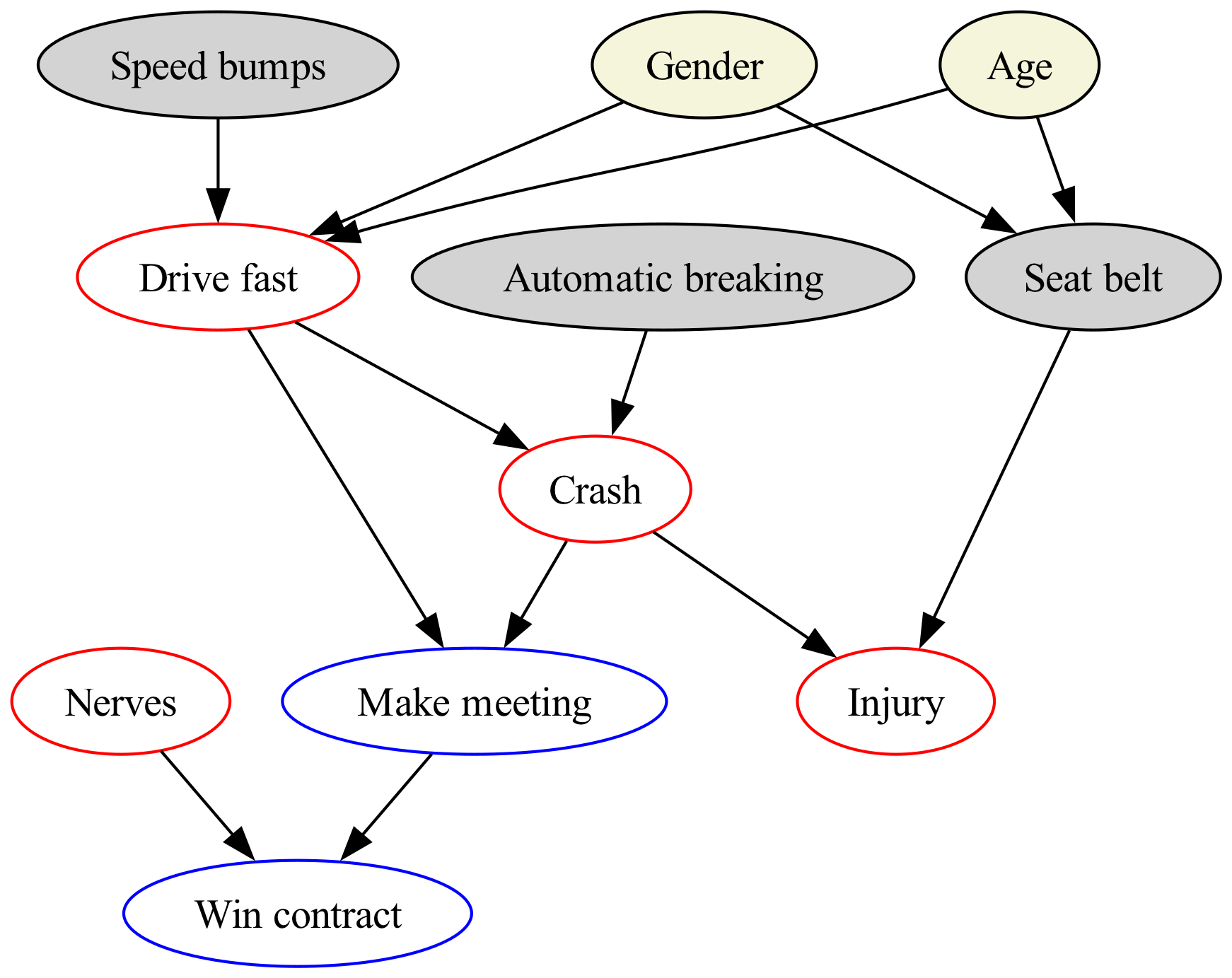
Figure 4 depicts the unified DAG that integrates driver motivation into a holistic, improved public health program theory. We cannot emphasize enough the importance of building causal graphs from multiple perspectives that include risks and benefits, and different strategy levels. This DAG is a big improvement.

Figure 4: Unified causal model that includes driver’s perspective (benefit-seeking) and program theory (risk-reduction)

However, when you review it with subject matter experts they suggest adding “gender” and “age” nodes because both are causally associated with driving fast and wearing seat belts (Figure 5). This will enable you to evaluate the effectiveness of the public health intervention while controlling for the confounding effects of gender and age. For example, if drivers are predominately young males (who drive fast and do not wear seat belts) then the seat belt intervention may appear falsely ineffective. These DAGs encode expert and community knowledge and wisdom, and are used for causal, evidential, and decision reasoning.

Figure 5: Expanded unified causal model with age and gender

If we would like to know if one of our interventions (e.g., seat belt use) is working we need to design a study or analysis to test our hypothesis. Unfortunately, without a causal model (Figure 5) to guide us, we cannot know what variables are required to test our intervention, and what variables to control for (“confounders”) that threaten the validity of our conclusions.

Here is a summary of program theory:

1. Every intervention has a program theory (whether expressed or not).

2. Program theory includes theories of causation, change, and action.

3. DAGs have archetypes: risk (adverse) event and benefit (opportunity) event.

4. Always include multiple causal perspectives (other causal drivers).

5. Use DAGs for root cause analyses and program theory design.

6. Don’t forget to consider confounders (that threaten validity).

7. Use DAGs to test interventions and to control confounding.

Getting this right is important because future decisions and resource allocations depends on these causal inferences. Understanding the basics of program theory is foundational.

Appendix (optional)

There are many ways to construct DAGs for visual display. In this case, I used Graphviz — an open source graph visualization software. At the command line I used for each figure:

dot -Tpng -Gdpi=300 sourcefile.gv -o outputfile.png

Figure 1

digraph ci {

rankdir=TB;

subgraph risk {

T [label="Trigger", color=red];

R [label="Risk event", color=red];

Con [label="Consequence", color=red];

T -> R [weight=10]

R -> Con [weight=10]

}

subgraph opp {

T2 [label="Trigger", color=blue];

R2 [label="Benefit event", color=blue];

Con2 [label="Consequence", color=blue];

T2 -> R2 [weight=10];

R2 -> Con2 [weight=10];

}

}

Figure 2

digraph ci {

rankdir=TB;

subgraph tocause {

T [label="Drive fast", color=red];

R [label="Crash", color=red];

Con [label="Injury", color=red];

T -> R [weight=10];

R -> Con [weight=10];

}

subgraph tochange {

P [fillcolor=lightgrey,style=filled,label="Speed bumps"];

P2 [shape=plaintext,label="Prevention Strategy"];

Ctrl [fillcolor=lightgrey,style=filled,label="Automatic breaking"];

Ctrl2 [shape=plaintext,label="Control Strategy"];

M [fillcolor=lightgrey,style=filled,label="Seat belt"];

M2 [shape=plaintext,label="Mitigation Strategy"];

P -> Ctrl -> M [style=invis];

P -> T

Ctrl -> R

M -> Con

P -> P2 [style=invis];

Ctrl -> Ctrl2 [style=invis];

M -> M2 [style=invis];

{rank=same; P2 P}

{rank=same; Ctrl2 Ctrl}

{rank=same; M2 M}

}

}

Figure 3

digraph ci {

rankdir=TB;

subgraph tocause {

T [label="Drive fast", color=red];

R [label="Make meeting", color=blue];

Con [label="Win contract", color=blue];

T -> R [weight=10];

R -> Con [weight=10];

}

subgraph tochange {

Ctrl [label="Crash", color=red];

Ctrl2 [shape=plaintext,label="Impediment"];

M [label="Nerves", color=red];

M2 [shape=plaintext,label="Impediment"];

Ctrl -> M [style=invis];

Ctrl -> R

M -> Con

Ctrl -> Ctrl2 [style=invis];

M -> M2 [style=invis];

{rank=same; Ctrl2 Ctrl}

{rank=same; M2 M}

}

}

Figure 4

digraph ci {

rankdir=TB;

df [label="Drive fast", color=red];

mm [label="Make meeting", color=blue];

wc [label="Win contract", color=blue];

cr [label="Crash", color=red];

in [label="Injury", color=red];

nn [label="Nerves", color=red];

P [fillcolor=lightgrey,style=filled,label="Speed bumps"];

Ctrl [fillcolor=lightgrey,style=filled,label="Automatic breaking"];

sb [fillcolor=lightgrey,style=filled,label="Seat belt"];

df -> mm -> wc

df -> cr -> in

cr -> mm

nn -> wc

P -> df

Ctrl -> cr

sb -> in

//{rank=same; df P}

}

Figure 5

digraph ci {

rankdir=TB;

df [label="Drive fast", color=red];

mm [label="Make meeting", color=blue];

wc [label="Win contract",color=blue];

cr [label="Crash", color=red];

in [label="Injury", color=red];

nn [label="Nerves", color=red];

P [fillcolor=lightgrey,style=filled,label="Speed bumps"];

Ctrl [fillcolor=lightgrey,style=filled,label="Automatic breaking"];

M [fillcolor=lightgrey,style=filled,label="Seat belt"];

Age [fillcolor=beige,style=filled,label="Age"];

Sex [fillcolor=beige,style=filled,label="Gender"];

df -> mm -> wc

df -> cr -> in

cr -> mm

nn -> wc

P -> df

Ctrl -> cr

M -> in

Age -> df

Age -> M

Sex -> df

Sex -> M

}

Footnotes

1. Funnell, Sue C., and Patricia J. Rogers. Purposeful Program Theory: Effective Use of Theories of Change and Logic Models. 1st ed. San Francisco, CA: Jossey-Bass, 2011.

2. DAGs are also called causal graphs.

3. Pearl, Judea, and Dana Mackenzie. The Book of Why: The New Science of Cause and Effect. First trade paperback edition. New York: Basic Books, 2020. For an introduction to causal inference and causal graphs, this book is HIGHLY RECOMMENDED.

4. Fenton, Norman E., and Martin Neil. Risk Assessment and Decision Analysis with Bayesian Networks. Second edition. Boca Raton: CRC Press, Taylor & Francis Group, 2019.